Analysis of VISGP result in R
We mapped the expression pattern of the SV genes based on R language and some R software packages.
Import packages
library(ggplot2)
library(gridExtra)
library(grid)
Load data
count <- read.csv("./data/Layer2_BC_expression.csv")
rownames(count) <- count[,1]
count <- as.data.frame(as.matrix(count[,2:ncol(count)]))
colnames(count) <- paste0("s",1:ncol(count))
info <- read.csv("./data/Layer2_BC_location.csv")
info <- as.data.frame(as.matrix(info[,2:ncol(info)]))
rownames(info) <- paste0("s",1:nrow(info))
Define function
# anscombe variance stabilizing transformation: NB
var_stabilize <- function(x, sv = 1) {
  varx = apply(x, 1, var)
  meanx = apply(x, 1, mean)
  phi = coef(nls(varx ~ meanx + phi * meanx^2, start = list(phi = sv)))
  return(log(x + 1/(2 * phi)))
}

# Linear normalization
relative_func <- function(expres){
  maxd = max(expres)-min(expres)
  rexpr = (expres-min(expres))/maxd
  return(rexpr)
}

# Plot gene expression pattern
pattern_plot <- function(pltdat, igene, xy=T, main=F, title=NULL) {
  if (!xy) {
    xy <- matrix(as.numeric(do.call(rbind, strsplit(as.character(pltdat[,1]), split = "x"))), ncol = 2)
    rownames(xy) <- as.character(pltdat[, 1])
    colnames(xy) <- c("x", "y")
    pd <- cbind.data.frame(xy, pltdat[, 2:ncol(pltdat)])
  } else {
    pd <- pltdat
  }
  pal <- colorRampPalette(c("mediumseagreen", "lightyellow2", "deeppink"))
  gpt <- ggplot(pd, aes(x=x, y=y, color=pd[, igene + 2])) + geom_point(size=4) +
    scale_color_gradientn(colours = pal(5)) + scale_x_discrete(expand=c(0, 1)) +
    scale_y_discrete(expand=c(0, 1)) + coord_equal() + theme_bw()
  if (main) {
    if (is.null(title)) {
      title = colnames(pd)[igene + 2]
    }
    out = gpt + labs(title=title, x=NULL, y=NULL) +
      theme(legend.position="none", plot.title=element_text(hjust=0.5, size=rel(1.5)))
  } else {
    out = gpt + labs(title=NULL, x=NULL, y=NULL) + theme(legend.position="none")
  }
  return(out)
}
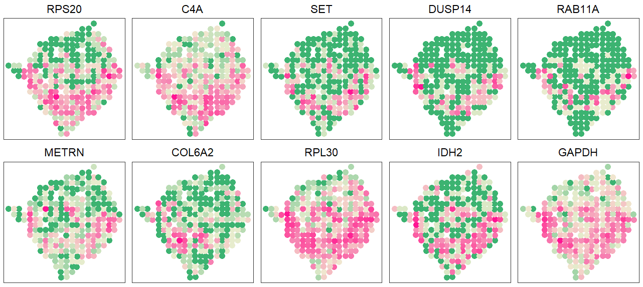
Plot gene expression pattern
count <- var_stabilize(count)
pltdat  <- cbind.data.frame(info[, 1:2], apply(count[c("GAPDH", "IDH2", "RPL30", "COL6A2", "METRN", "RAB11A", "DUSP14", "SET", "C4A", "RPS20"),], 1, relative_func))
plot <- lapply(1:10, function(x){pattern_plot(pltdat, x, xy = T, main = T)})
grid.arrange(grobs=plot[10:1], ncol=5)